electromagnetism - Calculating equipotential lines and current density in a rectangular conductor

(This isn't homework, I'm trying to make an illustration for an article I'm writing.)

Let's say that I have a thin rectangular bar of uniform conductivity, and I have point probes at various places:

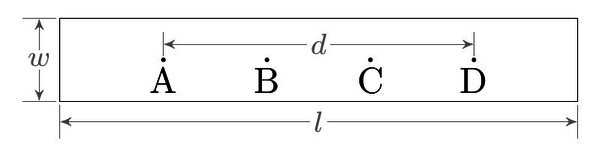
The bar has width $w$ and thickness $t$ where $t \ll w$. I am going to inject current into the bar between points $\boldsymbol A$ and $\boldsymbol D$. (let's just say 1 ampere enters at point $\boldsymbol A$ and leaves at point $\boldsymbol D$) These are centered along the bar's width and are a distance $d$ apart.

How would I figure out the equipotential lines and current density?

---

edit: Vague memories of college electrostatics are coming back - it's Laplace's equation that is relevant here, I need to find a solution to $\nabla^2 V = 0$, then the electric fields are just the gradient of $V$ so $J = \sigma E = \sigma \nabla V$, and I know the boundary conditions at the outside of the rectangle are that the perpendicular component of $E$ is $0$, but I'm not sure what to do next.

Answer

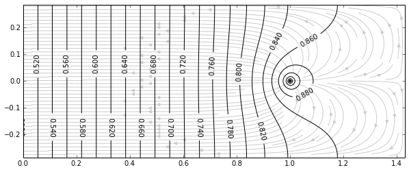
I solved my problem numerically, using the diffusion equation $\frac{\partial V}{\partial t} = -k\nabla^2 V$, with the following boundary conditions:

• Voltage at point D is fixed at 1.0


• Voltage along the vertical line halfway between points A and D is fixed at 0.5 (voltage at point A is 0.0, use symmetry so we don't have to simulate the left half of the material)


• The other three boundaries have the Neumann condition where the gradient of potential has zero component perpendicular to the boundary. For a rectangular array, this just means setting the top and bottom rows and the right column equal to their nearest neighbors off the boundary.

Iterate a bunch of times until equilibrium is reached and $\frac{\partial V}{\partial t} = 0$.

Then I graphed a streamplot and contour plot in matplotlib to show the current density and equipotentials:

This seems like it would be a well-known problem, though, and I'd be happier understanding an analytic solution that uses sums of the form $A_{mn} \sinh \frac{2m\pi x}{l} \cos \frac{2n\pi y}{w}$ or whatever.